Motivation for extension
The parameters of the equivalent circuit, \(p\), need to be calculated such that the impedance of the circuit, \(Z(f,p)\) is “equal” to the target impedance, \(Z_{tgt}(f)\). Since the impedance cannot always be made exactly equal, it is instead more practical to minimize the difference between the impedances instead. To this end
where the cost function,
The original impedance.py uses curve_fit (which uses least_squares under the hood), and basinhopping when global_opt=True. least_squares is well suited for functions with a single minimum. If there are multiple minima, least_squares may get stuck at a local minimum; as such it is sensitive to initial conditions. basinhopping primarily uses local gradient methods to find the (local) minimum. The algorithm then uses a “hop” to perturb the parameter, and then checks if the cost function could have a logical global trend. Hence, the basinhopping works well if cost-function has “funnel” of “bowl” topology with some “pits”.
We observed that basinhopping did not converge when data was noisy data. Hence, impedance_extend adds Particle Swarm Optimization (PSO) and Genetic Algorithm (GA) based optimization.
PSO works when the cost-function land scape is “Rugged & Noisy” with non-differentiable mountain range with many small, disconnected “false valleys,”.
GA works well when the cost-function landscape has local minimum with “Strong Local Attraction.”. Since GA spans the parameter space it is likely to reach the true minimum.
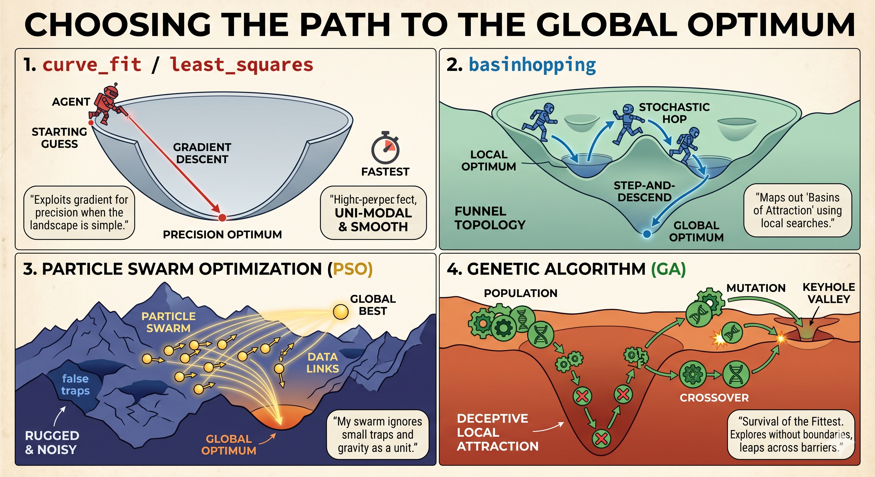
Illustration of the different optimization algorithms (AI generated).
Plevris et al. 10.21105/joss.02349 may provide better insights into the optimization problem (providing a head-to-head comparison between GA and PSO-based optimization and classical optimization for a wide rage of multi-parameter functions).
Additionally, impedance_extend adds exact Jacobian to the parameters and an option to disable runtime checks. Sample fitting for R0-p(R1,C1)-p(R2-Wo1,C2) indicates that the use of exact Jacobian can decrease least_squares fitting time by a factor of 5 (i.e. a 5-fold speed-up). Additionally, disabling run time checks (while not recommended) can decrease fitting time by a factor of 2 for all algorithms.